Electric field along axis with two charged rings

Example 1 Equal Charge Rings - Equal Radii- Both rings have the same charge .. just move them apart - away from the origin - and see how the net field changes.

Introduction : In discussing the electric field between (and away from) two charged rings along the X axis .. we started playing "battle of the rings" to see where the E field would be zero .. and if that would be a stable point or not. We use the convention that we plot the electric field pointing right on the the +y axis, and the electric field pointing left on the -y axis. Assume a single positively charged ring at the origin. We use the standare equation for the electric field along the axis from a charged ring - as shown to the right.

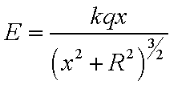
General shape of the curve? This will create an electric field that points right, on the right side of the ring, and points left on the left side, with a zero point at the middle of the ring (x=0). Now, since, from far away, this ring will "look like" a point charge, there must be a local maximum at some distance out from the ring on each side. If we solve for that location, we find it to be = R/sqrt(2). To the right is a picture of the general shape of the curve. [Note, in this picture, the radius of the ring is 3*sqrt(2) units, so the peak occurs at x=3 .]

Equilibrium Points? If the electric field is zero at a point along the axis, there will be no force on a test charge placed there (regardless of the sign of the test charge). But, if we move the test charge away from that point slightly, either it will want to return (stable) or it will want to keep going away (unstable). Using our plotting convention, the slope of the E curve, as it crosses that E=0 point, indicates which sign of the test charge will be unstable : that is, if the slope is positive, then a positive test charge will find that an unstable equilibrium point, but a negative test charge will find it a stable equilibrium point, and vice versa. Notice, that so far, there is only one zero point .. at the origin of the ring - and this will be unstable for postitive test charges (since the slope is positive). If you move a test charge slightly away from the ring, it will continue to move away!

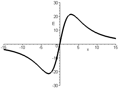
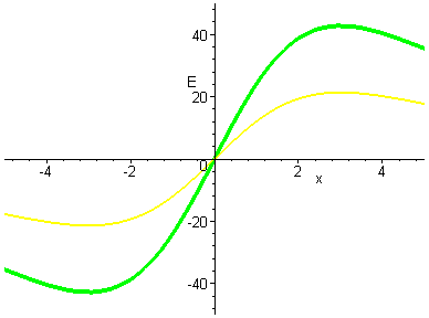
Two rings? To make it more interesting, let's have two charged rings, but to make it easier on ourselves, let's have the both the same radius and the same charge. In this case, if we have them separated by a distance, there will still be a point exactly between them where the Electric field is zero .. and eqilibrium point. First, we tried moving the rings a little bit apart ... and we got a modified field picture, but seemed reasonable (and the center, the slope was still positive). (Note that the blue curve is the left ring, at 2 units behind the origin, and the yellow curve is the right ring, at 2 units in front of the origin ... the Green is the net electric field.)

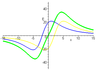
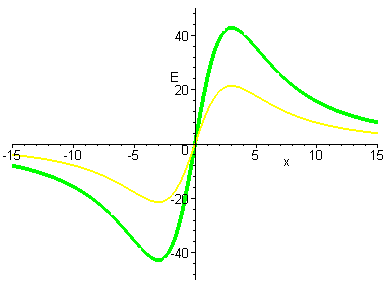
Move the rings farther apart? But, as we moved the rings farther apart ... the curve shifted to a negative slope! Here is an example.

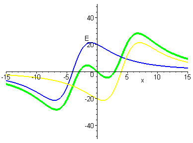
Animation of moving the rings? The next logical question is .. where is that crossover, and what does it look like?.

Here is an animation of the large scale view as we move from superimposed to a distance of 12 units out for each ring (thus the origin is always the zero point for the system - but we see other zeros show up!).

Close up view of what happens at the center?
When exactly does the change occur? It turns out when the maximum from one ring is at the origin, and the maximum of the other ring is at the origin (so in this case, when one ring is at x=-3, and the other is at x=+3, there will be an inflection point at the origin. .. Then the slope will switch signs!) This means that the + test charge unstable point, if the rings are close together, has become a stable point (if the rings are farther apart). Here is an animation of the zoomed in view view as we move from superimposed to a distance of 5 units out for each ring (in steps of 0.5 units). (The animation pauses at the "magic moment".)
[Notice that two more zeros appear .. both are unstable for the + test charge .. it could "squeeze out" of the system at those points (see the explanation below).]

What is a conceptual understanding of this changeover? Well, think of it this way .. if there is one ring, the center is an unstable point for a + test charge .. it wants to escape if it moves slightly away from the ring. Now, as you start to separate the rings, both are pushing at that + test charge, so you might think it would be held there, but, if it moves a little closer to one of the rings, the electric field actually decreases relative to that ring, and since it is moving farther from the other ring, that contribution also decreases .. so it says, "hey, I can escape!". Now, if the rings move farther apart, so that the place where the test charge is located will be beyond the "local maximum" of the individual rings, now if the test charge moves closer to one ring, it is fighting a bigger electric field, thus it wants to stay put ... STABLE!

How did I create these images? This was the problem that forced me to sit down and play around with Maple. I had to learn how to put in the equations, and get the plots that I wanted. To create the above animated gifs, I just exported out a series of images, and then used GifAnimator to string them together. (Maple has the ability to kick out an animated gif from an animation, I think .. but I haven't gotten that far yet!). If you want the simple file I used to generate these pictures, download this file [By that, I mean right-click on this link and save the file .. if you click the link you'll get a glorious page of "junk text"!] . I've tested it on Maple 5.1 and Maple 6.0.

It takes 37 licks to get to the center of a Tootsie Pop?